This is a shortened documentation of my undergraduate thesis—Keyword Spotting Using Convolutional Neural Network on Microcontroller-based Board as a Smart Switch for Devices. Basically, the prototype provided in the thesis is a voice-controlled smart switch for two devices. The trigger keywords are one, two, on, and off. One and two are used to switch between the two devices, while on and off, quite intuitively, are used to turn the devices on or off. Here is a demonstration video of the prototype. For clarification, all computation is performed on board. No external processors/computers were used to perform the keyword spotting algorithm. This means that the prototype has the potential of being a smartwear device that can control multiple devices remotely, especially that the board also has a BLE chipset.

Proceeding to the discussion of terms for easier discussion, keyword spotting (KWS) is a machine learning algorithm that is used to detect certain keywords from a stream of live audio. As for convolutional neural network (CNN), it is used in KWS to classify the keywords, CNN is a deep learning architecture commonly used for image classification. Lastly, microcontroller (MCU) is an embedded device found in almost all of commonly used electronic gadget, it can be simply described as a less-powerful miniature version of a computer. Arduino is a common development board that uses microcontroller.

Materials

Arduino Nano 33 BLE Sense

Arduino Nano 33 BLE Sense (Arduino 33) is an AI-enabled board—where AI-enabled means that it is compatible with existing AI software tools such as TensorFlow Lite for Microcontroller and Edge Impulse, etc.—operating at 3.3 V. It has multiple built-in sensors such as 9-axis inertial sensor, humidity and temperature sensor, barometric sensor, microphone, gesture sensor, proximity sensor, and light color and intensity sensor. It also has a Bluetooth Low Energy (BLE) chipset and can also be used as a Bluetooth host and client [1]. The pin diagram of Arduino 33 is shown below.

This board was selected due to its compatibility with existing Tiny Machine Learning frameworks and its availability.

Photo from [1]

Methods

Data Preprocessing

First off is a brief description of the data. Two datasets—speech commands dataset (SCD) v2 [2] and ESC-50 [3]—was combined in the study. Both datasets are audio/sound, with SCD created for the purpose of keyword spotting while ESC-50 for environmental classification. SCD has multiple keywords such as digits one to nine, activation words such as on and off, and some random words such as Marvin and Sheila. On the other hand, ESC-50 is a dataset composed of environmental sounds such as rain, clapping sounds, and cricket sounds.

To properly combine the datasets, ESC-50 was preprocessed as the same specifications of the SCD dataset. A script was written using python, so that ESC-50 samples are one-second length each and sampled at 16kHz. These samples were added to the background noise samples of the SCD. In preparing the dataset, a script was written to separate the keywords one, two, on, off, and background noise into a separate folder. Classes/labels in SCD not belonging to the prior mentioned keywords are randomly grouped into one label—unknown. The data distribution is uniform, each with 2500 samples, thus a total of 15,000 samples.

Feature Extraction

Audio is transformed into MFCC as the input to the CNN. This is done since CNN is commonly used in images (which are 2D signals) and audio is a 1D signal thus feature extraction is first performed on audio to convert it into 2D signal. Shown below is the process of MFCC conversion from audio of Edge Impulse. To extract MFCC, Edge Impulses uses SpeechPy, a Python package for extracting features from audio by Torfi [4].

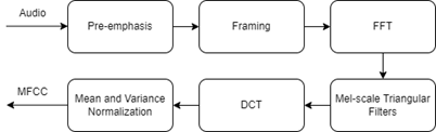
MFCC is a signal processing function offered by Edge Impulse which converts raw audio data into mel-frequency spectrogram. Shown below is a pictorial process of the conversion.

CNN Model Selection

Three models are adapted for this study’s use-case. These models should have small-footprint and low computation time. The application should also be sound/voice classification. To make the process easier, CNN models that have already been deployed to Arduino 33 are more preferred as opposed to models deployed on other microcontroller-based boards.

The first model is from Waqar et al [5], which is used for Speech Emotion Recognition (SER). The audio data is converted to MFCC, which is then used as the input for the CNN. The SER The SER application of the study is on anger classification, where they used 0.98 confidence as “angry”, 0.55 to 0.98 as “about to be angry” and less than 0.55 as “not angry”. The trained model was deployed onto Arduino 33. The model architecture is shown in Figure 3-7a.

The second model is from Amjath and Kuhanesan [6], which is a warning system for railway track workers, they named TrackWarn. The input used for the study is also MFCC. The model is a binary classification, with 0.7 confidence to be classified as the train sounds. The trained model was deployed to Arduino 33. The architecture is shown in Figure 3-7b.

Lastly, the third model is from Trivedi and Shroff [7], which classifies three species of mosquitoes based on the sound of their wing beats. The input used for the study is Mel-Filterbank Energy, which is like MFCC, except DCT was not performed. The trained model was deployed to Arduino 33 using Edge Impulse. The architecture is seen in Figure 3-7c.

The input shape for models is the size of the extracted MFCC, ℝ1 x 650. All the convolution layers use ReLu as the activation layer. The output of the max pooling/last convolutional layer is flattened, followed by dropout (randomly dropping nodes to address overfitting) before going to the output layer with activation of SoftMax. The optimizer to be used is Adam optimizer, and the loss function is categorical cross entropy.

Hyperparameter Optimization

Since the models selected have different datasets and applications, the hyperparameters included in their study may not work properly on the use-case of KWS. Additionally, the dataset used in this study is also different from what the models used. Furthermore, the models selected also used different input size in comparison to what is used in the study.

To address the prior problems, the hyperparameters need to be optimized to improve the performance of the models for this study’s application. This is implemented using Keras-Tuner, with their built-in RandomSearch algorithm.

The hyperparameters tuned were dropout rates 1 and 2, learning rate, and batch size. For hyperparameters such as dropout rate and learning rate which are both float types, method Float() is used. For batch size, which are usually in powers of 2, an array is provided, which elements are chosen randomly and uniformly. The neural network is trained for 120 epochs.

To compensate for the high epoch of 120 (in terms of computation time), Early Stopping is used, which stops the training of a neural network when the objective is not improving after n iterations, where n is the patience value set by the user. The objective used in this study is the validation accuracy with patience of 10. The objective is the validation accuracy since the test set is not included in the hyperparameter optimization (to avoid the hyperparameters being biased towards the test set).

The top three models for each architecture are trained on Edge Impulse, where the best model (out of the nine models) is the model that is deployed to Arduino 33. Models are retrained on Edge Impulse because it currently has no feature for deploying models trained outside of Edge Impulse.

Shown below is the hyperparameter search space of Mosquito and Trackwarn

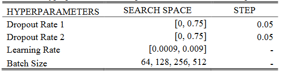
while below is Waqar

Model Training and Deployment via Edge Impulse

After hyperparameter tuning, the top three models for each architecture (Waqar, Mosquito, and TrackWarn) was retrained on Edge Impulse. Edge Impulse uses Keras to train neural networks. However, since MCUs are restricted with their low memory and computational power. TensorFlow Lite for Microcontrollers is used to quantize the models. Using full-integer quantization significantly reduces memory usage by 62.96%.

Proceeding to the results, shown below are the hyperparameters of the top nine performing models. TrackWarn Rank 1 (F1 score of .893) and Waqar Rank 2 (F1 score of .888) are considered as the models to be deployed. Comparing their F1 scores, TrackWarn Rank 1 is the better model, with percent difference of 0.56% or difference of 0.5% (as they are both percentage). However, considering the theoretical inference time, Waqar Rank 2 has a faster inference time, with percent difference of about 2% between the two models. This is where the tradeoff between performance and computation time is considered, TrackWarn Rank 1 has better accuracy and performance of about 0.6% while Waqar Rank 2 has a faster inference computation time of about 2%. For the use-case of this study, a higher F1 score is preferred than faster inference time, thus TrackWarn Rank 1 is used. However, TrackWarn Rank 1 is only selected because the difference of the inference is only 2%, which is a small number considering the inference time is in milliseconds (in this case, about 0.5ms). If the percent difference between the two is to be 10- 15% and the F1 score difference remained the same, Waqar Rank 2 will be selected.

Evaluation of the deployment model shows that quantization caused an increase in accuracy, as opposed to the usual decrease. This might be due to the representative dataset used in the full integer quantization of the model. A full integer quantization requires a representative dataset which is a small subset of the dataset. This is used to estimate the input and output tensor since they are variable, compared to weights. The quantization process might have used a representative dataset that had a better/more biased portrayal of the dataset.

Since the deployment model is picked, next then is deploying the model onto Arduino 33. This is easily done in Edge Impulse because they use TensorFlow Lite for Microcontrollers, which is used in quantizing models so they consume less memory. Especially since MCU-based boards have low memory and computational power.

MFCC Classification Analysis

The MFCC of incorrect classifications can also be analyzed to determine why the model has the wrong predictions for some of the samples. Shown in Appendix F are 10 samples of On, Off, One, and Two; five properly classified, and five misclassified. It could be observed from the Off samples that a certain pattern can be inferred from the correctly classified samples. The patterns are boxed green below, which is colored dark red to light red from rows (coefficient axis) 0 to 3, with length of around 16-25 in the columns (time axis). This pattern is followed by low energy shown as color blue. By listening to the audio of the samples, it could be deduced that the darker red part is the “o-“ sound while the lighter red is the “-ff” sound, which are then followed by silence.

Evaluating the misclassified samples, the first MFCC looks like an “off” sound that immediately gets cut off. The second and third MFCC has no visible patterns forming which means it could just be noise. For the fifth, the pattern looks like “o-“ which means the time-shift of the audio exceeded the window, and the “-ff” sound was cut-off. Finally, the fourth sample looks like the MFCCs of the correct classifications. Verifying the patterns of the misclassified samples by listening to the audio, MFCC 1, 2, 4, 5 has correct hypotheses. However for MFCC 3, an “a-“ sound is heard instead of noise. This might be an Off sample that was cut-off due to wrong time-shift. MFCC 2, 3, and 5 was misclassified because it was not a correct Off sample. The mislabeling might be due to improper data preprocessing (e.g., too much time-shift) or it might have been mislabeled by the person who labeled the data. For MFCC 1, it could be hypothesized that the network only learned the correct Off classification from Off samples followed by silence, hence the Off pattern from MFCC 1 being at the edge caused the network to misclassify it. However, MFCC 4 is a correct Off sample, and the MFCC formed looks similar to correctly classified MFCCs. The only difference might be that the pattern has a lighter shade of red in the front, in comparison to the correct MFCCs with dark red color at the beginning of the red line.

On-board inferencing

Continuous audio inferencing

To perform continuous inferencing, the input data are first stored into smaller sampling buffers (slices) which are then passed into the inferencing algorithm. The slices are sequentially placed into a First In First Out (FIFO) buffer which has the size of the input audio used in the model (in this study is one second). These slices are converted into features (this algorithm is also part of the inferencing process), specifically MFCC and then classified. Signal processing and inferencing is done in slices because it takes a lot of resources (in terms of computation time), where it takes as much as 500ms to compute the MFCC for a 1000ms window, with this method, no windows are overlapping thus it could miss some utterance of the keywords. Thus, it is more efficient to perform 49 feature extraction on each slice, put them into the FIFO buffer, and classify the whole second of data [8-9]. Below is a flowchart of the algorithm from [8]

Photo from [8]

Smart switch algorithm

For the smart switch algorithm, shown below is a flowchart. State variables are used (Boolean type), which are is_one and is_two. Both are initialized as false, and they are only assigned true when the classifier returns a score of greater than 0.6 for labels One and Two respectively. These state variables are mutually exclusive.

If is_one is true, LED 1 can be turned on or off when the classifier returns a score greater than 0.6 for labels “on” or “off” respectively. LED 2 similarly also has this algorithm but instead uses state variable is_two. A change in state, for example, is_one changes from true to false, means that is_two is now true (because they are mutually exclusive) and the user can now control LED 2. However, this does not mean that the state of LED 1 also changes, the prior state of the LED is retained even if the state variables change. For example, LED 1 is on, then state variable is_two is now true, LED 1 cannot be controlled anymore but it remains on and can only be turned off by uttering “one” and “off”. Below shows the snippet of the Arduino code from Edge Impulse, showing the algorithm for the smart switch. buzzer_one and buzzer_two is just an indicator for is_one and is_two. It could also be replaced with an LED.

References

[1] https://store-usa.arduino.cc/products/arduino-nano-33-ble-sense

[2] https://arxiv.org/abs/1804.03209

[3] https://dl.acm.org/doi/10.1145/2733373.2806390

[4] https://zenodo.org/record/840395

[5] https://ieeexplore.ieee.org/document/9526323

[6] https://ieeexplore.ieee.org/document/9568329

[7] https://ieeexplore.ieee.org/document/9662116

[8] https://docs.edgeimpulse.com/docs/tutorials/continuous-audio-sampling

[9] https://forum.edgeimpulse.com/t/question-about-regular-vs-continuous-classification/3889